Correlation energy and excitation spectrum

This example shows how to compute the correlation energy and excitation spectrum for a system of two polarizable units (oscillators).

General preparations

First we import the necessary modules and prepare a hypothetical system with a response represented by a Casida matrix. The response of, e.g., molecules or nanoparticles is managed via Response objects. In this example, we consider different synthetic oscillators, the response of which is described by a set of randomized Casida matrices as obtained via build_random_casida. This is useful for demonstration purposes only. In practice, one would rather use the response of a real system as obtained from, e.g., TDDFT calculations via GPAW or NWChem, which can be parsed via builder functions.

import matplotlib.pyplot as plt
import numpy as np
from pandas import DataFrame
from strongcoca import CoupledSystem, PolarizableUnit
from strongcoca.calculators import CasidaCalculator
from strongcoca.response import build_random_casida

# Set up a the response of a hypothetical system based on a Casida matrix
# description
response = build_random_casida(n_states=3, name='Grizzly', random_seed=42)

Resonant oscillators as a function of distance

We can now investigate the variation of the correlation energy and the excitation spectrum with distance for a system of two polarizable units that have individually the same response. The polarizable units are represented by objects of the PolarizableUnit class and are both initialized using the same build_random_casida function, which means they have the same underlying response function. After the two units have been added to an object of the CoupledSystem class, a CasidaCalculator is set up to work on the coupled system response. Its get_correlation_energy methods and excitations attribute allow one to obtain and inspect the correlation energy and the spectrum of the coupled system. The positions (and orientations, see below) of the underlying polarizable units can be changed directly via the position property of the PolarizableUnit.

# We construct a coupled system from two polarizable units with the same
# response functions.
pu1 = PolarizableUnit(response, [0, 0, 0])
pu2 = PolarizableUnit(response, [1.5, 0, 0])
cs = CoupledSystem([pu1, pu2])

# Now we set up a calculator and compute the spectrum and correlation energy
# as a function of the distance between the units.
calc = CasidaCalculator(cs)
data = {}
for dr in np.arange(2.0, 6.0, 0.02):
    pu2.position = [dr, 0, 0]
    ecor = calc.get_correlation_energy()
    excitations = calc.excitations.energies
    data[dr] = {'energy': ecor}
    data[dr].update({f'excitation{k}': en for k, en in enumerate(excitations)})
df = DataFrame.from_dict(data).T

For convenience the results are stored as a pandas DataFrame object and plotted using matplotlib.

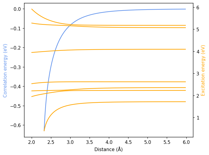
The results show the resonant coupling of the two system with bonding and anti-bonding modes arising from the combination of resonant excitations. Below we show the correlation energy (blue) and the excitation energies (orange) for a system of two resonant oscillators as a function of distance.

fig, ax = plt.subplots()
ax.plot(df.energy, color='cornflowerblue')
ax.set_xlabel('Distance (Å)')
ax.set_ylabel('Correlation energy (eV)', color='cornflowerblue')
ax.set_ylim((-0.37, 0.02))
ax2 = ax.axes.twinx()
for fld in df.columns:
    if 'excitation' not in fld:
        continue
    ax2.plot(df[fld], color='orange')
ax2.set_ylabel('Excitation energy (eV)', color='orange')
ax2.set_ylim(0, 6)
fig.tight_layout()

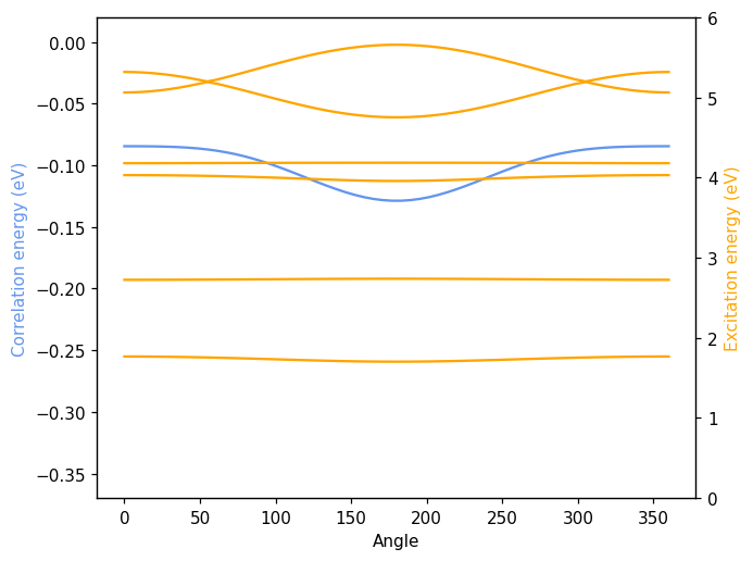
Resonant oscillators as a function of rotation angle

We can furthermore investigate the changes in the aforedescribed system as one of the two polarizable units is rotated. To this end, we modify the orientation of the second unit, which can be done using set_orientation.

Plotting proceeds as before.

# We repeat the above exercise but this time one of the polarizable units is
# being rotated while the distance is kept constant.
pu1 = PolarizableUnit(response, [0, 0, 0])
pu2 = PolarizableUnit(response, [3, 0, 0])
cs = CoupledSystem([pu1, pu2])
calc = CasidaCalculator(cs)
data = {}
for ang in np.linspace(0, 360, 60):
    pu2.set_orientation(rotation_axis=[1, 0, 0],
                        rotation_angle=ang,
                        units='degrees')
    ecor = calc.get_correlation_energy()
    excitations = calc.excitations.energies
    data[ang] = {'energy': ecor}
    data[ang].update({f'excitation{k}': en for k, en in enumerate(excitations)})
df = DataFrame.from_dict(data).T

fig, ax = plt.subplots()
ax.plot(df.energy, color='cornflowerblue')
ax.set_xlabel('Angle')
ax.set_ylabel('Correlation energy (eV)', color='cornflowerblue')
ax.set_ylim((-0.37, 0.02))
ax2 = ax.axes.twinx()
for fld in df.columns:
    if 'excitation' not in fld:
        continue
    ax2.plot(df[fld], color='orange')
ax2.set_ylabel('Excitation energy (eV)', color='orange')
ax2.set_ylim(0, 6)
fig.tight_layout()

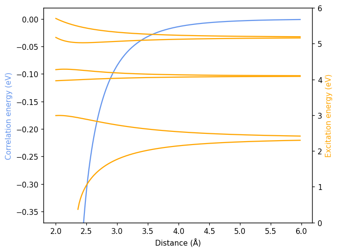
Non-resonant oscillators as a function of distance

Finally, we demonstrate what happens if we repeat the above exercise using two non-resonant oscillators. To this end, we set up two different response functions and then repeat the calculation of the correlation energy and the spectrum as a function of distance.

response1 = build_random_casida(n_states=3, name='Grizzly', random_seed=42)
response2 = build_random_casida(n_states=4, name='Polar bear', random_seed=43)
pu1 = PolarizableUnit(response1, [0, 0, 0])
pu2 = PolarizableUnit(response2, [1.5, 0, 0])
cs = CoupledSystem([pu1, pu2])
calc = CasidaCalculator(cs)
data = {}
for dr in np.arange(2.0, 6.0, 0.02):
    pu2.position = [dr, 0, 0]
    ecor = calc.get_correlation_energy()
    excitations = calc.excitations.energies
    data[dr] = {'energy': ecor}
    data[dr].update({f'excitation{k}': en for k, en in enumerate(excitations)})
df = DataFrame.from_dict(data).T

fig, ax = plt.subplots()
ax.plot(df.energy, color='cornflowerblue')
ax.set_xlabel('Distance (Å)')
ax.set_ylabel('Correlation energy (eV)', color='cornflowerblue')
ax2 = ax.axes.twinx()
for fld in df.columns:
    if 'excitation' not in fld:
        continue
    ax2.plot(df[fld], color='orange')
ax2.set_ylabel('Excitation energy (eV)', color='orange')
fig.tight_layout()