The dipolar coupling method

In this tutorial we use strongcoca to calculate optical spectra of a coupled nanoparticle-molecule assembly. The method is described in the theory section on dipolar coupling. As inputs, the individual polarizabilities of the units are required.

We obtain the polarizability of benzene via the Casida TDDFT approach, using the NWChem code. The hybrid exchange-correlation functional B3LYP is used to obtain accurate molecular excitations.

The benzene_monomer.out.gz is the compressed output file from the calculation. The output file also contains a copy of the input file used to run the calculation. Strongcoca can read this file using the read_nwchem_casida function. Additionally, we need to provide a value and type of broadening, for which we specify 0.1 eV of LorentzianBroadening. We load the file and print the response object to verify that it contains 16 excited states between 5.5 and 9.0 eV.

from strongcoca.response import read_nwchem_casida
from strongcoca.response.utilities import LorentzianBroadening

broadening = LorentzianBroadening(0.1)
mol_response = read_nwchem_casida('benzene_monomer.out.gz', broadening=broadening)
print(mol_response)

---------------------- CasidaResponse ----------------------
name           : NWChem Casida Response
n_states       : 16
D (eV)         : [5.49336 6.2029  7.09528 ... 8.16819
                  9.03567 9.04532]
K (eV)         : [[0. 0. 0. ... 0. 0. 0.]
                  [0. 0. 0. ... 0. 0. 0.]
                  [0. 0. 0. ... 0. 0. 0.]
                  ...
                  [0. 0. 0. ... 0. 0. 0.]
                  [0. 0. 0. ... 0. 0. 0.]
                  [0. 0. 0. ... 0. 0. 0.]]
mu (eÅ)        : [[-3.17506e-04  0.00000e+00 -0.00000e+00]
                  [ 0.00000e+00 -6.66763e-04 -5.29177e-06]
                  [-5.29177e-06  1.05835e-05 -0.00000e+00]
                  ...
                  [-0.00000e+00  0.00000e+00 -0.00000e+00]
                  [-0.00000e+00 -0.00000e+00  5.29177e-06]
                  [ 1.58753e-05  1.58753e-05  0.00000e+00]]
broadening     : LorentzianBroadening(0.1, units='eV')
atoms          : C6H6

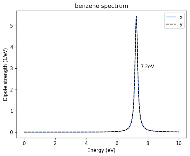
We check the response of the molecule by plotting the absorption spectrum, expressed as the dipole strength function. The spectrum is degenerate in x and y directions, with the first bright state at 7.2 eV.

import matplotlib.pyplot as plt
import numpy as np

frequencies = np.linspace(0, 10, 200)
absorption = mol_response.get_dipole_strength_function(frequencies)

fig, ax = plt.subplots()
ax.plot(frequencies, absorption[:, 0], color='cornflowerblue', label='x')
ax.plot(frequencies, absorption[:, 1], color='k', ls='--', label='y')
ax.set(xlabel='Energy (eV)', ylabel='Dipole strength (1/eV)',
       title='benzene spectrum')
ax.legend()

# Find the peak
peakfreq = frequencies[np.argmax(absorption[:, 0])]
ax.annotate(f'{peakfreq:.1f}eV', (peakfreq + 0.3, 3));

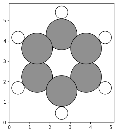
Since the output file contains the atomic structure, strongcoca also reads this structure as an ASE Atoms object. We can visualize it using ASE.

from ase.visualize.plot import plot_atoms

plot_atoms(mol_response.atoms);

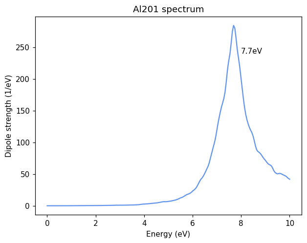
The polarizability of the nanoparticle can be computed using RTTDDFT, as this method scales better for large systems than the Casida method. We will use one of the Al NPs from Rossi et al. (2019), as these Al NPs have their localized surface plasmon resonance (LSPR) close to the first excitation of benzene. The Al201_dm.dat file contains the time-dependent dipole moment for a 201-atom regular truncated octahedron structure. The data was generated using the GPAW code and the original data files and scripts generating the data can be found on Zenodo.

We read the dipole moment file using the read_gpaw_tddft function. If we want to visualize the structure, we also need to pass the name of the atomic structure file Al201.xyz to this function.

We print the response and plot the absorption spectrum, which is isotropic, to find the LSPR at 7.7 eV.

from strongcoca.response import read_gpaw_tddft
from strongcoca.response.utilities import LorentzianBroadening

broadening = LorentzianBroadening(0.1)
NP_response = read_gpaw_tddft('Al201_dm.dat', atoms_file='Al201.xyz',
                              broadening=broadening)
print(NP_response)

frequencies = np.linspace(0, 10, 200)
absorption = NP_response.get_dipole_strength_function(frequencies)

fig, ax = plt.subplots()
ax.plot(frequencies, absorption[:, 0], color='cornflowerblue')
ax.set(xlabel='Energy (eV)', ylabel='Dipole strength (1/eV)',
       title='Al201 spectrum')

# Find the peak
peakfreq = frequencies[np.argmax(absorption[:, 0])]
ax.annotate(f'{peakfreq:.1f}eV', (peakfreq + 0.3, 240));

-------------------- TimeDomainResponse --------------------
name                : GPAWTDDFT
times (fs)          : [0.0000e+00 1.5000e-02 3.0000e-02 ...
                       2.9970e+01 2.9985e+01 3.0000e+01]
dipole_moments (eÅ) : [[[  0.        0.        0.     ]
                        [  0.        0.        0.     ]
                        [  0.        0.        0.     ]]

                       [[187.55988   0.        0.     ]
                        [  0.      187.55988   0.     ]
                        [  0.        0.      187.55988]]

                       [[365.46465   0.        0.     ]
                        [  0.      365.46465   0.     ]
                        [  0.        0.      365.46465]]

                       ...

                       [[  8.99014   0.        0.     ]
                        [  0.        8.99014   0.     ]
                        [  0.        0.        8.99014]]

                       [[ 14.1917    0.        0.     ]
                        [  0.       14.1917    0.     ]
                        [  0.        0.       14.1917 ]]

                       [[ 18.98371   0.        0.     ]
                        [  0.       18.98371   0.     ]
                        [  0.        0.       18.98371]]]
broadening          : LorentzianBroadening(0.1, units='eV')
atoms               : Al201

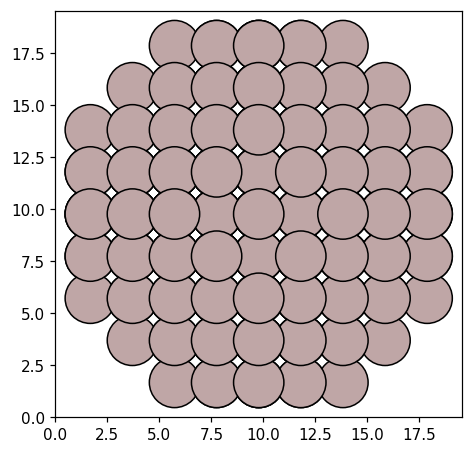
If we included the structure file, then we can also plot the structure.

plot_atoms(NP_response.atoms);

Coupled system

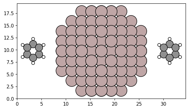
Now, we can construct the coupled system, by placing the one benzene molecule, one Al NP, and another benzene molecule on a line along the x-axis.

Each system is represented by a PolarizableUnit, which takes an position and Response object. We set up the units of our system, and add them to a CoupledSystem, which represents the full system. Placing the center of mass of the benzene structure at \(\pm 14\) Å and the NP at the origin, the distance between the edges of the NP and the nearest molecule is about 3 Å.

Having added the atomic structures to the response objects, we can display the atomic structure of the CoupledSystem. This is useful to verify that the units are positioned and rotated according to our expectations.

Note

Structures can be rotated by strongcoca using one of the orientation_kwargs to the PolarizableUnit constructor.

from strongcoca import CoupledSystem, PolarizableUnit

pus = [PolarizableUnit(mol_response, [-14, 0, 0]),  # Benzene at -14 Å
       PolarizableUnit(mol_response, [+14, 0, 0]),  # Benzene at +14 Å
       PolarizableUnit(NP_response, [0, 0, 0]),  # NP at the origin
      ]
cs = CoupledSystem(pus)

plot_atoms(cs.to_atoms());

Now, we calculate the spectrum of the coupled system using the dipolar coupling method, which is implemented in the PolarizabilityCalculator. To set up the calculator, we need the CoupledSystem and a grid of frequencies used for integration along the imaginary axis. Since we do not intend to use this feature, we can leave a dummy grid of [0, 1].

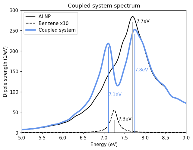
Plotting the absorption spectrum of the coupled system from the calculator, we see the emergence of two new peaks. This is a signature of strong coupling. The new resonances are polaritons, which are hybrid states of the localized surface plasmon in the NP and the molecular excitation. The lower polariton has a frequency of 7.1 eV and the upper 7.8 eV.

In Fojt et al. (2021), a comparison can be found between spectra obtained using the dipolar coupling method and TDDFT, showing where the regime where the method works well and where it breaks down.

from strongcoca.calculators import PolarizabilityCalculator

calc = PolarizabilityCalculator(cs, [0, 1])

frequencies = np.linspace(5, 9, 200)
NP_absorption = NP_response.get_dipole_strength_function(frequencies)
mol_absorption = mol_response.get_dipole_strength_function(frequencies)
coupled_absorption = calc.get_dipole_strength_function(frequencies)

fig, ax = plt.subplots()
ax.plot(frequencies, NP_absorption[:, 0], color='k',
       label='Al NP')
ax.plot(frequencies, 10 * mol_absorption[:, 0], color='k', ls='--',
       label='Benzene x10')
ax.plot(frequencies, coupled_absorption[:, 0], color='cornflowerblue',
       label='Coupled system', lw=3)
ax.set(xlabel='Energy (eV)', ylabel='Dipole strength (1/eV)',
       xlim=[5, 9], ylim=[0, 300], title='Coupled system spectrum');
ax.legend()

# Find the peaks
peakfreq = frequencies[np.argmax(mol_absorption[:, 0])]
ax.annotate(f'{peakfreq:.1f}eV', (peakfreq + 0.1, 30));
ax.axvline(peakfreq, ymax=0.1, color='0.7')

peakfreq = frequencies[np.argmax(NP_absorption[:, 0])]
ax.annotate(f'{peakfreq:.1f}eV', (peakfreq + 0.1, 270));
ax.axvline(peakfreq, ymax=0.9, color='0.7')

# Upper polariton
peakfreq = frequencies[np.argmax(coupled_absorption[:, 0])]
ax.annotate(f'{peakfreq:.1f}eV', (peakfreq, 150), color='cornflowerblue');
ax.axvline(peakfreq, ymax=0.8, color='cornflowerblue')

# Lower polariton
peakfreq = frequencies[np.argmax(coupled_absorption[frequencies < 7.3, 0])]
ax.annotate(f'{peakfreq:.1f}eV', (peakfreq, 90), color='cornflowerblue');
ax.axvline(peakfreq, ymax=0.7, color='cornflowerblue');

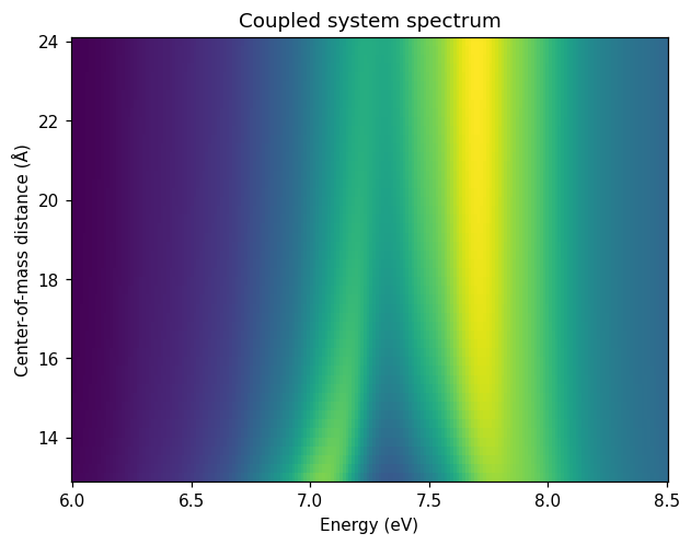
Since the dipolar coupling method is very fast, we can afford to perform many calculations, sweeping the distance parameter. We end up with a map of the spectrum, where the emergence of the two polaritons from the underlying excitations is seen around 16 Å center-of-mass distance.

from strongcoca import CoupledSystem, PolarizableUnit

distances = np.linspace(13, 24)
frequencies = np.linspace(6, 8.5, 200)
spectra = []

for dist in distances:
    pus = [PolarizableUnit(mol_response, [-dist, 0, 0]),
           PolarizableUnit(mol_response, [+dist, 0, 0]),
           PolarizableUnit(NP_response, [0, 0, 0]),
          ]
    cs = CoupledSystem(pus)

    calc = PolarizabilityCalculator(cs, [0, 1])

    spectra.append(calc.get_dipole_strength_function(frequencies)[:, 0])  # x

fig, ax = plt.subplots()
ax.pcolormesh(frequencies, distances, spectra, cmap='viridis', rasterized=True)
ax.set(xlabel='Energy (eV)', ylabel='Center-of-mass distance (Å)',
       title='Coupled system spectrum');

References

•  T. P. Rossi, T. Shegai, P. Erhart, and T. J. Antosiewicz, Strong plasmon-molecule coupling at the nanoscale revealed by first-principles modeling, Nat. Commun. 10 (2019).

•  J. Fojt, T. P. Rossi, T. J. Antosiewicz, M. Kuisma, and P. Erhart, Dipolar coupling of nanoparticle-molecule assemblies: An efficient approach for studying strong coupling, J. Chem. Phys. 154 (2021).