Mie-Gans response

For an ellipsoid of a solid material in vaccum there is an analytic expression for the polarizability in the dipolar limit (Sihvola (2007)). This is known as the Mie-Gans solution. For an ellipsoid with semi-axes \(a_x\), \(a_y\), \(a_z\) along the Cartesian directions, and the dielectric function \(\varepsilon(\omega)\) of the material and the dielectric constant \(\varepsilon_m\) of the environment, the polarizability is diagonal

\[\alpha_{\mu\mu}(\omega) = \varepsilon_0 V \frac{\varepsilon_r(\omega) - \varepsilon_m}{\varepsilon_m + N_\mu (\varepsilon_r(\omega) - \varepsilon_m)},\]

where \(N_\mu\) are the depolarization factors

\[N_\mu = \frac{a_x a_y a_z}{2} \int_0^\infty \frac{\mathrm{d}s}{(s+a_\mu^2)\sqrt{(s+a_x^2)(s+a_y^2)(s+a_z^2)}}\]

and the volume of the particle is

\[\frac{4\pi}{3} a_x a_y a_z.\]

For the special case of a sphere, the depolarization factors \(N_\mu\) are \(1/3\). In vacuum (\(\varepsilon_m\) = 1) the polarizability is

\[\begin{align} \alpha(\omega) = 3\varepsilon_0 V \frac{\varepsilon(\omega) - 1}{\varepsilon(\omega) + 2}. \end{align}\]

It is useful to keep in mind that in Hartree atomic units the vacuum permitivity is \(\varepsilon_0 = \frac{1}{4\pi}\) Then the polarizability of a general ellipsoid is

\[\alpha_{\mu\mu}(\omega) = \frac{a_x a_y a_z}{3} \frac{\varepsilon_r(\omega) - \varepsilon_m}{\varepsilon_m + N_\mu (\varepsilon_r(\omega) - \varepsilon_m)}.\]

The polarizability of a sphere of radius \(r\) in vacuum is

\[\alpha(\omega) = r^3 \frac{\varepsilon_r(\omega) - 1}{\varepsilon_r(\omega) + 2}.\]

Reading the dielectric function

Using strongcoca, we can calculate the Mie-Gans response.

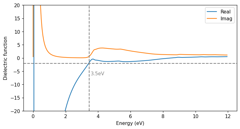
First, we retireve the dielectric function file of Ag dielectric_function_Pd_0.00_Ag_100.00.txt. This dielectric function is computed with TDDFT and is published with a library of dielectric functions (Rahm (2020)). The library is available online on SHARC.

Strongcoca can read this file using the read_dielec_function_file function. For a sphere, the resonance should occur where the real part of the denominator \(\mathrm{Re}\:\varepsilon(\omega) + 2\) is zero. We plot a horizontal line to mark \(\mathrm{Re}\:\varepsilon(\omega) = -2\) and see that this occurs at 3.5 eV.

import numpy as np
import matplotlib.pyplot as plt
from strongcoca.response import read_dielec_function_file

# Read Ag dielectric function (data from DFT)
df = read_dielec_function_file('dielectric_function_Pd_0.00_Ag_100.00.txt')

fig, ax = plt.subplots(1, 1, figsize=[8, 4])
ax.plot(df.frequencies, df.dielectric_function.real, label='Real')
ax.plot(df.frequencies, df.dielectric_function.imag, label='Imag')
ax.set(ylim=[-20, 20], ylabel='Dielectric function', xlabel='Energy (eV)')
ax.legend()

# Find resonance
ax.axhline(-2, ls='--', color='0.5')
index = np.argmax(df.dielectric_function.real[df.frequencies > 2] > -2)
resonance = df.frequencies[df.frequencies > 2][index]
ax.annotate(f'{resonance:.1f}eV', (resonance + 0.1, -5), color='0.5', va='top')
ax.axvline(resonance, ls='--', color='0.5');

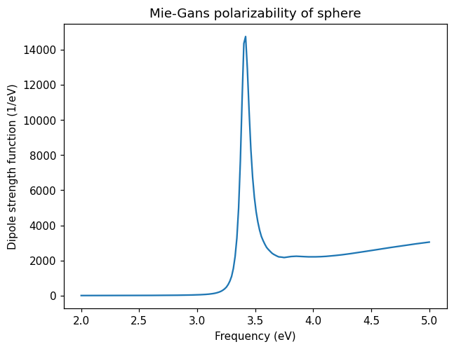
Obtaining the response

Now, we can calculate the response using a MieGansResponse object. To make a sphere, we only specify the radius (20 Å) and provide the dielectric function. The resonance is close to where we predicted from the \(\mathrm{Re}\:\varepsilon(\omega) = -2\) criterion. The reason that the resonance is not there exactly is due to the finite imaginary part of the dielectric function.

from strongcoca.response import MieGansResponse

response = MieGansResponse(50, df)  # Radius of 20Å

frequencies = np.linspace(2, 5, 200)
absorption = response.get_dipole_strength_function(frequencies)

fig, ax = plt.subplots(1, 1)
ax.plot(frequencies, absorption[:, 0])  # x-component
ax.set(xlabel='Frequency (eV)', ylabel='Dipole strength function (1/eV)',
       title='Mie-Gans polarizability of sphere');

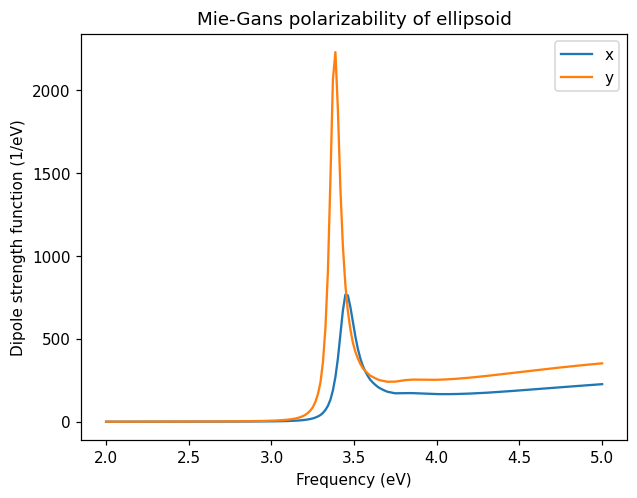
We can also calculate the response of an ellipsoid, by specifying the semiaxes as a list, instead of the radius.

The response of the ellipsoid is non-isotropic, and the longer axes have a redshifted resonance.

response = MieGansResponse([20, 25, 25], df)  # Semi-axes of (20, 25, 25)Å

frequencies = np.linspace(2, 5, 200)
absorption = response.get_dipole_strength_function(frequencies)

fig, ax = plt.subplots(1, 1)
ax.plot(frequencies, absorption[:, 0], label='x')
ax.plot(frequencies, absorption[:, 1], label='y')
ax.set(xlabel='Frequency (eV)', ylabel='Dipole strength function (1/eV)',
       title='Mie-Gans polarizability of ellipsoid')
ax.legend()

<matplotlib.legend.Legend at 0x7ff343228550>

References

•  A. Sihvola, Dielectric Polarization and Particle Shape Effects, J. Nanomater. (2007).

•  J. M. Rahm, C. Tiburski, T. P. Rossi, F. A. A. Nugroho, S. Nilsson, C. Langhammer, and P. Erhart, A Library of Late Transition Metal Alloy Dielectric Functions for Nanophotonic Applications, Adv. Funct. Mater. 30 (2020).